Exercice 13
| > | restart; |
| > | rho:=theta->(1+2*cos(theta))/(2*sin(theta)+1); |
![]()
Domaine d'Etude
On rÈduit l'intervalle d'Ètude ‡ -Pi..Pi par pÈriodicitÈ
| > | rho(theta+2*Pi)=rho(theta); |
![]()
| > | evalb(%); |
![]()
| > |
s
Points caractÈristiques
Intersection avec l'axe des abscisses
| > | assume(t>=-Pi and t<=Pi); |
| > | r:=[solve(rho(t)=0,t)]; |
avec le point O
![]()
| > | r:=[solve(rho(t)*sin(t)=0,t)]; |
avec l'axe des abscisses
![]()
| > | r:=[solve(rho(t)*cos(t)=0,t)]; |
avec l'axe des ordonnÈes
![]()
| > | t_0:=-2*Pi/3:M(t_0)=[rho(t_0)*cos(t_0),rho(t_0)*sin(t_0)],'rho'(t_0)=rho(t_0); |
![]()
| > | t_0:=-Pi/2:M(t_0)=[rho(t_0)*cos(t_0),rho(t_0)*sin(t_0)],'rho'(t_0)=rho(t_0); |
![]()
| > | t_0:=0:M(t_0)=[rho(t_0)*cos(t_0),rho(t_0)*sin(t_0)],'rho'(t_0)=rho(t_0); |
![]()
| > | t_0:=Pi/2:M(t_0)=[rho(t_0)*cos(t_0),rho(t_0)*sin(t_0)],'rho'(t_0)=rho(t_0); |
![]()
| > | t_0:=2*Pi/3:M(t_0)=[rho(t_0)*cos(t_0),rho(t_0)*sin(t_0)],'rho'(t_0)=rho(t_0); |
![]()
Calcul de la direction de la tangente
| > | Drho:=D(rho); |
![]()
| > | cV:=Drho(theta)/rho(theta); |

| > | cV:=factor(simplify(cV)); |
cotan V
![]()
| > | V:=unapply(arccot(cV),theta); |
On en dÈduit V modulo Pi
![]()
D'o˘ quelques tangentes particuliËres
| > | t_0:=-Pi/2:'V'(t_0)=V(t_0); |
![]()
| > | t_0:=0:'V'(t_0)=V(t_0); |
![]()
| > | t_0:=Pi/2:'V'(t_0)=V(t_0); |
![]()
les tangentes ont mÍme orientation relativement ‡ la direction (OM)
| > |
Etudions les asymptotes en -Pi/6 et -5Pi/6
| > | t_0:=-Pi/6:#En -Pi/6 ‡ droite, on a bien une branche infinie car: |
| > | Limit('rho'(theta),theta=t_0,right)=limit(rho(theta),theta=t_0,right); |
![]()
la direction asymptotique est -Pi/6.
dans le repËre tournÈ de cet angle on a la coordonnÈe Y
| > | Y:=theta->rho(theta)*sin(theta+Pi/6); |
![]()
| > | Limit('Y'(theta),theta=t_0,right)=limit(Y(theta),theta=t_0,right); |
![]()
D'o˘ l'Èquation de l'asymptote dans ce nouveau repËre Y=1+sqrt(3)/3
Position relative:
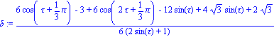
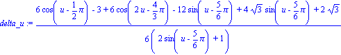
| > | delta:=simplify(combine(Y(tau)-1-sqrt(3)/3));#Expression de Y(tau)-1-sqrt(3)/3 |

| > | delta_u:=subs(tau=u-Pi/6,delta);#changement de variable |

| > | Limit('delta_u'/u,u=0,right)=limit(delta_u/u,u=0,right); |
![]()
Comme delta_u est au voisinage de 0 (‡ droite) du signe de la limite delta_u/u, on trouve que
la courbe est au dessus de l'asymptote
| > | u:='u':#assume(u>-Pi/6 and u<-Pi/7); |
| > | plot(delta_u,u=-0.1..0.1); |
![[Plot]](images/ex13_25.gif)
| > |
| > | t_0:=-Pi/6: |
En -Pi/6 ‡ gauche, on a bien une branche infinie car:
| > | Limit('rho'(theta),theta=t_0,left)=limit(rho(theta),theta=t_0,left); |
![]()
la direction asymptotique est -Pi/6. dans le repËre tournÈ de cet angle on a la coordonnÈe Y
| > | Y:=theta->rho(theta)*sin(theta+Pi/6); |
![]()
| > | Limit('Y'(theta),theta=t_0,left)=limit(Y(theta),theta=t_0,left); |
![]()
D'o˘ l'Èquation de l'asymptote dans ce nouveau repËre Y=1+sqrt(3)/3
Position relative:
| > | delta:=simplify(combine(Y(tau)-1-sqrt(3)/3));#Expression de Y(tau)-1-sqrt(3)/3 |

| > | delta_u:=subs(tau=u-Pi/6,delta);#changement de variable |

| > | Limit('delta_u'/u,u=0,left)=limit(delta_u/u,u=0,left); |
![]()
comme delta_u est au voisinage de 0 (‡ droite) du signe contraire de la limite delta_u/u, on trouve que
la courbe est en dessous de de l'asymptote
| > |
| > |
| > |
| > | t_0:=-5*Pi/6: |
En -5Pi/6 ‡ droite, on a bien une branche infinie car:
| > |
| > | Limit('rho'(theta),theta=t_0,right)=limit(rho(theta),theta=t_0,right); |
![]()
la direction asymptotique est -5Pi/6. dans le repËre tournÈ de cet angle on a la coordonnÈe Y
| > | Y:=theta->rho(theta)*sin(theta+5*Pi/6); |
![]()
| > | Limit('Y'(theta),theta=t_0,right)=limit(Y(theta),theta=t_0,right); |
![]()
D'o˘ l'Èquation de l'asymptote dans ce nouveau repËre Y=1-sqrt(3)/3
Position relative:
| > | delta:=simplify(combine(Y(tau)-1+sqrt(3)/3));#Expression de Y(tau)-1+sqrt(3)/3 |

| > | delta_u:=subs(tau=u-5*Pi/6,delta);#changement de variable |

| > | Limit('delta_u'/u,u=0,right)=limit(delta_u/u,u=0,right); |
![]()
comme delta_u est au voisinage de 0 (‡ droite) du signe de la limite delta_u/u, on trouve que
la courbe est en desous de l'asymptote
| > |
| > | t_0:=-5*Pi/6:#En -5Pi/6 ‡ gauche, on a bien une branche infinie car: |
| > |
| > | Limit('rho'(theta),theta=t_0,left)=limit(rho(theta),theta=t_0,left); |
![]()
| > | #la direction asymptotique est -Pi/6. dans le repËre tournÈ de cet angle on a la coordonnÈe Y |
| > | Y:=theta->rho(theta)*sin(theta+5*Pi/6); |
![]()
| > | Limit('Y'(theta),theta=t_0,left)=limit(Y(theta),theta=t_0,left); |
![]()
D'o˘ l'Èquation de l'asymptote dans ce nouveau repËre Y=1-sqrt(3)/3
Position relative:
| > | delta:=simplify(combine(Y(tau)-1+sqrt(3)/3));#Expression de Y(tau)-1-sqrt(3)/3 |
| > | delta_u:=subs(tau=u-5*Pi/6,delta);#changement de variable |
| > | Limit('delta_u'/u,u=0,left)=limit(delta_u/u,u=0,left); |
![]()
comme delta_u est au voisinage de 0 (‡ gauche) du signe contraire de la limite delta_u/u, on trouve que
la courbe est au dessus de de l'asymptote
| > |
| > |
| > |
Variations de rho et de V
| > | plot(rho,-Pi..Pi,-10..10,discont=true); |
![[Plot]](images/ex13_44.gif)
| > | plot(V,-Pi..Pi,discont=true); |
![[Plot]](images/ex13_45.gif)
| > |
Support de courbe
| > | total:=[rho(t),t,t=-Pi..Pi]:asymp1:=[rho(t),t,t=-Pi/6..0]:asymp2:=[rho(t),t,t=-Pi/2..-Pi/6]:asymp3:=[rho(t),t,t=-5*Pi/6.. -5*Pi/6+0.4]:asymp4:=[rho(t),t,t=-5*Pi/6-0.2..-5*Pi/6]: |
| > | plot([total,asymp1,asymp2,asymp3,asymp4],-2..5,-2..3,color=[red,blue,green,magenta,black],thickness=[2,2,2,2,2],coords=polar); |
![[Plot]](images/ex13_46.gif)
En bleu la partie asymptotique correspondant ‡ -Pi/6 ‡ droite (courbe au dessus? voir sens du vecteur v(-Pi/6))
En vert la partie asymptotique correspondant ‡ -Pi/6 ‡ gauche (courbe en dessous voir sens du vecteur v(-Pi/6))
En magenta la partie asymptotique correspondant ‡ -5Pi/6 ‡ droite (courbe en dessous voir sens du vecteur v(-5Pi/6))
En noir la partie asymptotique correspondant ‡ -5Pi/6 ‡ gauche (courbe au dessus voir sens du vecteur v(-5Pi/6))